Are Your Iceberg Writes Optimized?

If you have any of the following questions while working (more than just small POCs) with Apache Iceberg:
- Why did the run time increase after I migrated from Hive Table Format to Apache Iceberg Table Format? Wasn't it supposed to reduce? 🤔
- Why are my Spark Jobs creating huge or too many small files per partition?
- Why and when should I worry about controlling the file sizes?
- How do I control the file size during write times? Isn't that something that requires running compaction?
This post will explore all the key concepts and details to address these questions. By the end, you will gain a solid understanding of how Apache Iceberg functions and the important factors influencing write times.
Spark 3.5 and Iceberg 1.5.0Let's get into it..!!
from Tenor
Why does controlling file size matter?
A large number of small files can cause read query degradation, but a huge file can cause spills to disk during decompression, frequent GC, etc.
Both cases can result in overall job run time degradation if not avoided. Here's a quick summary of issues both the cases can cause:
Small Files
A large number of small files cause:
- Heavy network I/O Load, especially in the case of Cloud Object Storages like AWS S3, because of the overhead required to make multiple requests (like
List,Get, orHead) for many objects. - Read overhead, i.e., for any Query Engine to run a query, each file must be opened, scanned, and closed when done. The more files the query engine has to scan for a query, the more of a cost these file operations will put on your query.
Large Files
Reading too large files can result in:
- More CPU utilization to compress and decompress data.
- Spilling to disk during decompression if executor memory is not sufficient.
- Due to frequent Garbage Collection, GC Pressure can occur due to large object allocation and deallocation, leading to performance degradation.
This can also significantly increase the job run times while writing due to the time it takes to write a big compressed file.
Before moving forward, here is a quick recall of how Spark Job works internally – Every action invokes a Spark Job, Spark Jobs has Stages, and Stages has Tasks. These tasks are written as a file (one file/task) during write time.
Job >> Stages >> Tasks (n) >> n Files written
So, the main thing to understand from here is:
The file size on disk depends on the size of the Task being written as a file.
This means if the task size is 100MB in memory before writing into the table, the file written will always be < 100MB (due to compression used in file formats like Parquet, ORC, etc., before writing).
Concepts to understand
To understand these concepts, assume an Iceberg table that stores Taxi Trips data. It is partitioned by VendorId and has three distinct VendorIds: 1, 2, and 3.
Write Distribution Modes
Iceberg provides control over various aspects of the writing process.
This is achieved internally by using the connector API to request a specific distribution (Exchange) and ordering (Sort) for the incoming data. Distribution modes can be defined at
- Table Level by setting it in table properties –
write.distribution-mode - Spark Session Configuration using
spark.sql.iceberg.distribution-mode
Distribution modes set via Spark Session Configuration overwrites the one defined in Table Properties.
Before we dive deeper into how these distribution modes work, one more thing to know is that each Task present during the writing stage gets its own Iceberg Writer.
This means if Spark Stage has 3 tasks, there will be 3 writers performing writes in parallel compared to if there is a single task, i.e. no writes happening in parallel.
This can be seen in the SparkWrite.java class:
@Override
public DataWriter<InternalRow> createWriter(int partitionId, long taskId) {
  return createWriter(partitionId, taskId, 0);
}
Code Snippet from SparkWrite.java
Iceberg has 3 Write Distribution Modes:
Unspecified Distribution (write.distribution-mode = none)
Data in each task is written as it is, with no additional steps to align it with the table partitioning.
When VendorIds data is spread across several tasks - commonly seen when writing data to multiple partitions - it may create numerous small files in table partitions. This occurs because multiple Iceberg writers are writing to the same table partitions.
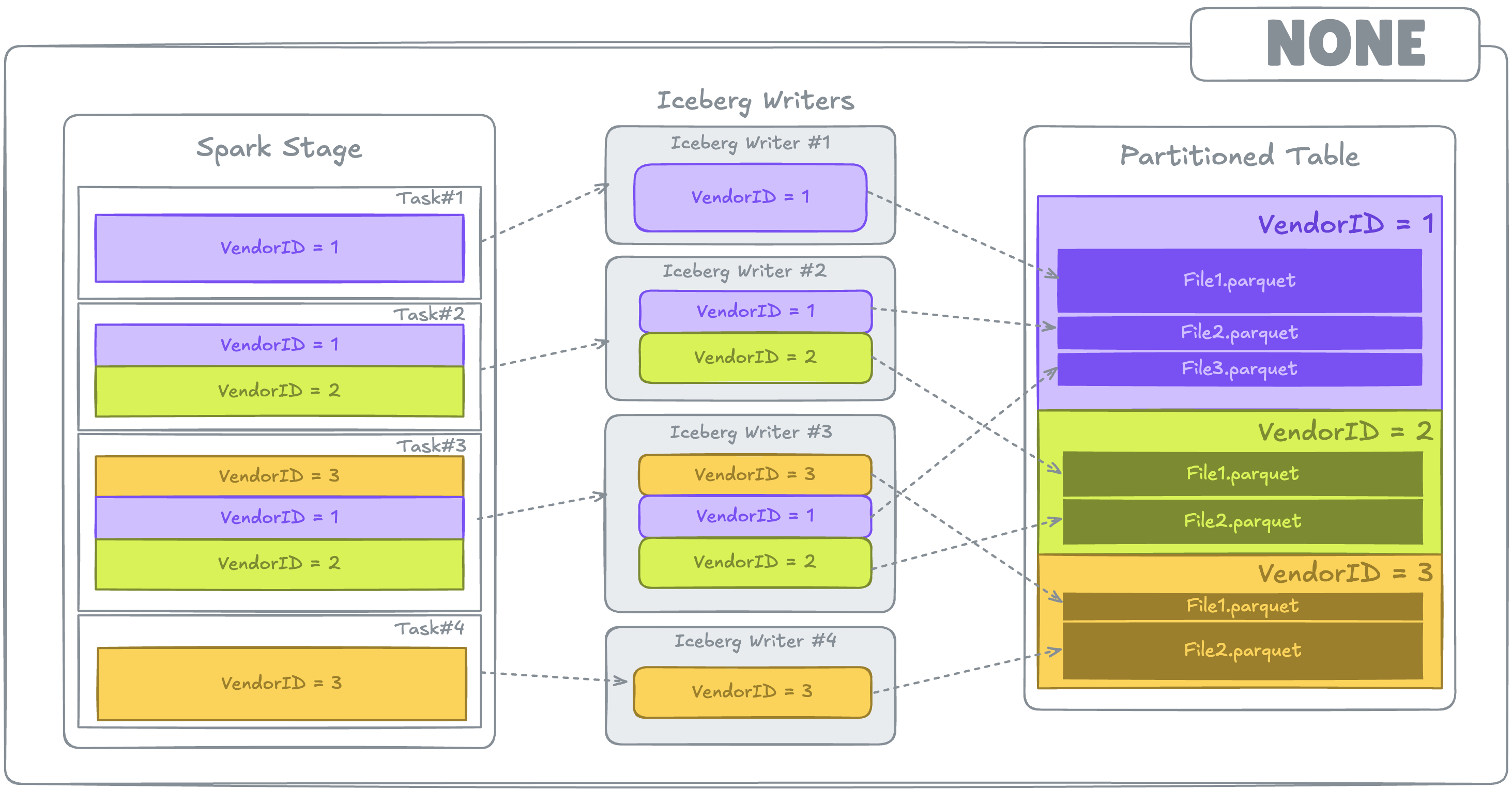
none. Colored boxes represent different partitions of data within a Task.Here's an example how Spark Plan looks like when none distribution mode is used:
spark.conf.set("spark.sql.iceberg.distribution-mode", "none")

plan = spark.sql(f"""EXPLAIN FORMATTED
			UPDATE {g_table}
			SET fare_amount=1.0
			WHERE fare_amount < 0 and VendorID = 1 and month=9
			""").collect()[0][0]
print(plan)
Write Distribution set as none via Spark Configuration
== Physical Plan ==
ReplaceData (4)
+- AdaptiveSparkPlan (3)
   +- Project (2)
      +- BatchScan local.nyc_tlc.green_taxi_trips (1)
Spark Plan when Write Distribution is set as none
More details later on when to use and when not to use this distribution mode.
Clustered Distribution (write.distribution-mode = hash)
Clustered Distribution guarantees that records sharing the same values for the clustering expressions (partitions in this scenario) are co-located to the same task.
Co-locating these records requires shuffling of data before write, i.e. this results in the addition of an Exchange Node before writes. Data is shuffled using HashPartitioner,i.e., it uses Spark Repartition by hash of partition values.
As a result of these shuffles, a Spark Task writes to a single Iceberg Partition (unless there are hash collisions, i.e., the hash of different partition values results in the same result).
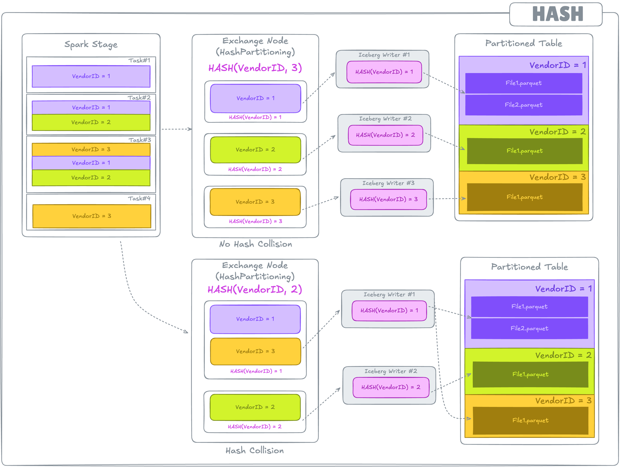
hash. Colored boxes represent different partitions of data within a Task.A hashpartitioning Exchange Node before write operation.This is the default mode. So, until and unless the distribution mode is changed, there will always be a shuffle happening before writes.
Here's how the Spark Plan will look like:
spark.conf.set("spark.sql.iceberg.distribution-mode", "hash")

plan = spark.sql(f"""EXPLAIN FORMATTED
			UPDATE {g_table}
			SET fare_amount=1.0
			WHERE fare_amount < 0 and VendorID = 1 and month=9
			""").collect()[0][0]
print(plan)
Write Distribution set as hash via Spark Configuration
== Physical Plan ==
ReplaceData (5)
+- AdaptiveSparkPlan (4)
   +- Exchange (3)
      +- Project (2)
         +- BatchScan local.nyc_tlc.green_taxi_trips (1)

(3) Exchange
Input [22]: [VendorID#1939, ....
Arguments: hashpartitioning(VendorID#2539, 200), REBALANCE_PARTITIONS_BY_COL, 268435456, [plan_id=1041]
Spark Plan when Write Distribution is set as hash. A hashpartitioning Exchange Node before writes.
Ordered Distribution (write.distribution-mode = range)
This distribution mode instructs Spark to range-partition the data being written, according to a given list of ordering expressions. It uses RangePartitioner,i.e., Spark Repartition by Range.
Spark RangePartitioner samples the entire dataset and then splits it into a range. This can result in a Spark Task containing data for multiple partitions. Sampling in this case is an expensive operation, but it also ensures ordering across output files for efficient queries.
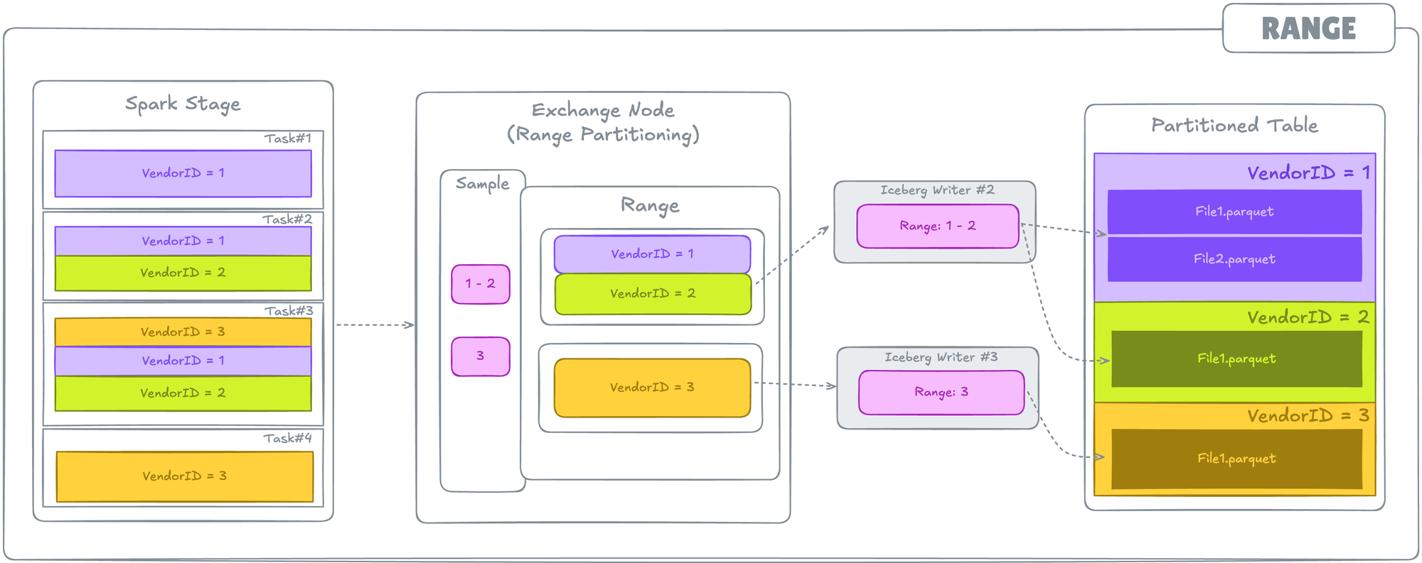
range. Colored boxes represent different partitions of data within a Task. A rangepartitioning Exchange Node before write operation.This mode is also used by default when a Sort Order is defined as an Iceberg Table Definition.
Here's how Spark Plan looks like:
spark.conf.set("spark.sql.iceberg.distribution-mode", "range")

plan = spark.sql(f"""EXPLAIN FORMATTED
			UPDATE {g_table}
			SET fare_amount=1.0
			WHERE fare_amount < 0 and VendorID = 1 and month=9
		""").collect()[0][0]
Write Distribution set as range via Spark Configuration
== Physical Plan ==
ReplaceData (5)
+- AdaptiveSparkPlan (4)
   +- Exchange (3)
      +- Project (2)
         +- BatchScan local.nyc_tlc.green_taxi_trips (1)

(3) Exchange
Input [22]: [VendorID#1939, ....
Arguments: rangepartitioning(VendorID#1939 ASC NULLS FIRST, 200), REBALANCE_PARTITIONS_BY_COL, 268435456, [plan_id=908]
Spark Plan when Write Distribution is set as range. A rangepartitioning Exchange Node before writes.
After understanding distribution modes, the most common notion that comes to mind (especially those who have worked with Spark long enough and are chasing job optimization):
- No shuffles in
nonemode!! That's nice, that's going to improve the job performance. I can just usenonefor everything. - Why would I use the
hashdistribution mode, when it introduces a shuffle before write? Why would I want to do that? Shuffles are expensive. rangedistribution mode – um... No Thanks...!!
Before I get into all of these and burst some bubbles, let's understand 2 more configurations and how these work.
Configurations
Apache Iceberg provides some configurations that can help in controlling the file size.
write.target-file-size-bytes
This defines the size of the file written on disk. Default: 512MB
For instance, if the table file format is Parquet, this configuration defines the size of the compressed Parquet files generated after the job completes.
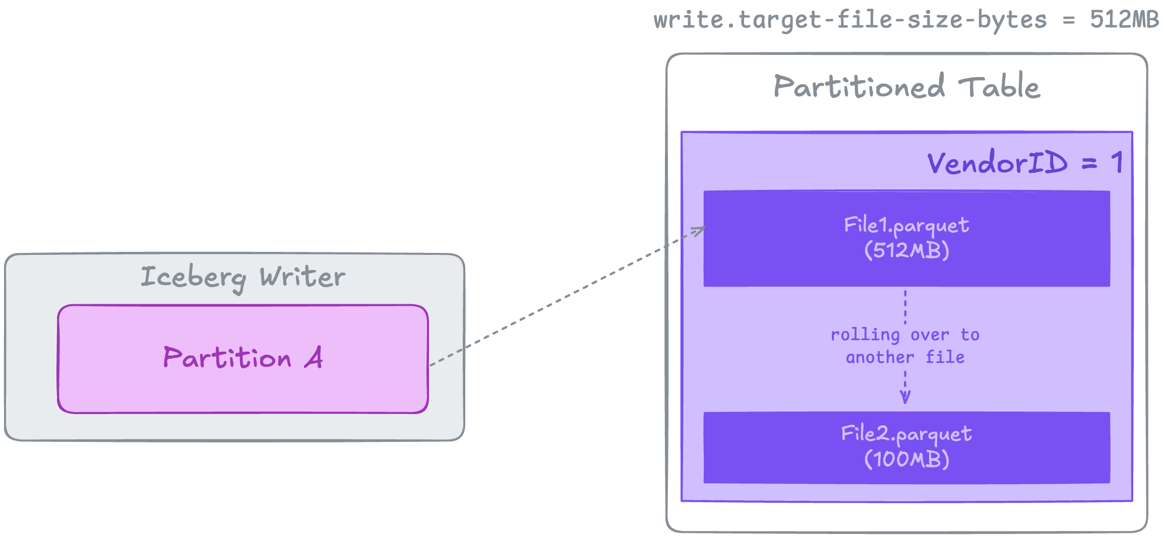
write.target-file-size-bytesAs illustrated above, if an Iceberg Writer has a Partition containing data that is compressed to more than 512MB on disk, it will result in the creation of two Parquet files. One of these files will have a size of 512MB, while the other will contain the remaining data.
A Note on Iceberg Writers
Iceberg Writers are implemented as RollingDataWriters for physically writing all file formats except ORC. This rolling writer creates a new data file whenever the number of buffered records exceeds the threshold defined by write.target-file-size-bytes.
This raises a very common question by the Data Engineers – Why isn’t my Spark Job writing a single file in Iceberg Table, despite defining this configuration at the table level? Instead, Spark writes multiple files.
At this point, you might already know the answer to this if you have followed the content so far – Size of generated files are capped by the in-memory Task Size that is being written.
In simpler words, if Spark Write Stage has 3 tasks of 100MB data each, Spark can't write just one file of 30MB (assuming 10x compression). Remember, each task gets it's own Iceberg writer (assuming all tasks has same VendorId data), in this case 3 writers and hence 3 files of 10MB each.
spark.sql.iceberg.advisory-partition-size
This defines the in-memory task size before writing the data into an Iceberg Table.
Below illustration shows the process when advisory-partition-size is set to 128MB and data in a task of Spark Stage before writing > 128MB.
During the last shuffle before write, Iceberg rebalances the in-memory partition based on the 128MB per partition/task size.

iceberg.advisory-partition-sizeIceberg Advisory Partition Size shouldn't be confused with Spark's AQE advisoryPartititionSizeInBytes defined via spark.sql.adaptive.advisoryPartitionSizeInBytes.
Um... What's the difference?
- AQE advisory partition size (further referred as APS) is the shuffle partition size during AQE optimization. It takes effect when Spark coalesces small shuffle partitions or splits skewed shuffle partition.
- Iceberg APS takes effect only before the writes happening to Iceberg Tables. Updating this doesn't impact the shuffle partition size being used by AQE anywhere else.
For Iceberg APS to work, it requires a Shuffle Stage to be present before the write, i.e., distribution-mode has to behashorrange.
As a matter of fact, we can actually see this in Spark Plan also, in case you haven't noticed earlier.
== Physical Plan ==
ReplaceData (5)
+- AdaptiveSparkPlan (4)
   +- Exchange (3)
      +- Project (2)
         +- BatchScan local.nyc_tlc.green_taxi_trips (1)

(3) Exchange
Input [22]: [VendorID#1939, ....
Arguments: hashpartitioning(VendorID#2539, 200), REBALANCE_PARTITIONS_BY_COL, 268435456, [plan_id=1041]
If you notice the Exchange details in the plan, REBALANCE_PARTITIONS_BY_COL, 268435456, the number 268435456 tells what partition size Iceberg APS is aiming for, i.e., 268435456=256MB
Adjusting AQE APS impacts the entire job shuffle partitions size (i.e., it will impact all the joins/aggregation/AQE optimization triggers), while, Iceberg APS only impacts the shuffle partition size in the shuffle before writing.
Before we throw everything into the mix and answer all the questions we begin with, one last thing (I promise), let's look at AQE because we can't leave it out when shuffling is involved.
Spark's Adaptive Query Execution (AQE)
AQE optimizes queries primarily after the shuffle or broadcast exchange stages, which are collectively known as “query stages.” These stages serve as materialization points for collecting runtime statistics.
While AQE offers various optimizations, only Dynamic Coalesce Partitioning and Splitting Skewed Partition are relevant in the context of Iceberg distribution mode.
- Splitting Skewed Partition: Skewed partitions are handled by breaking these down into smaller partitions.
- Dynamic Coalesce Partitioning: Smaller partitions are coalesced together to create a single partition.
Now, if you are wondering, Okay so if AQE is triggered after Exchange stages, in case of hash and range distribution, it makes sense that there is an AdaptiveSparkPlan after Exchange node in the Spark plans for these distribution.
Why is AdaptiveSparkPlan mentioned in the case of none distribution, since there’s no Exchange node involved?
Bravo!!👏 Great Question. I had the same question so I did some digging and here is the reason for that:
When there are no Exchange or broadcast nodes, AQE does not perform runtime re-optimization, because there are no materialization points to collect statistics[1][2]. The AdaptiveSparkPlan node is present, but it acts as a pass-through: the plan is not adaptively changed at runtime.
The presence of AdaptiveSparkPlan does not guarantee that adaptive optimizations will occur. It simply means the plan is eligible for AQE. Actual runtime adaptation only happens if there are Exchange (shuffle/broadcast) or subquery nodes, which enable Spark to collect statistics and re-optimize the plan.Combining everything together
Time to combine all the concepts altogether, and burst some bubbles.
Remember, there’s no one-size-fits-all solution in Data Engineering. So, feel free to run your own tests and benchmarking as needed. This section is here to give you a solid foundation to handle issues you might be facing during writes.
When to use which distribution and their impacts on write performance?
To make it easier to explain and understand, let's consider the scenario where our jobs are writing data into a single table partition (reason being, explanation here can be expanded across multiple partitions too easily).
Here's the scenario:
- An Iceberg Table partitioned on
year - Ingests NYC Taxi data in Parquet format for
year=2023. (Compressed Parquet File Size:1GB)
#1 Distribution Type = none
As mentioned before, with none distribution mode there will be no shuffling before write.
- Number of files depends on the number of tasks present during the Spark Write Stage.
- If there is only
1Task with all the data that needs to be written into table:- No shuffle requirement before write – NO AQE comes into action at this stage.
- No impact of setting
spark.sql.iceberg.advisory-partition-size(referred asAPSfurther) as it requires a shuffle to work. - There will be total of 2 files written sequentially –
512 MBeach. Defaultwrite.target-file-size-bytes = 536870912 (512 MB)[3] - This sequential writes can result in longer write times.
- If there are
Nnumber of tasks with data spread across all of these:- No shuffle – NO AQE optimization to coalesce the smaller partitions
Nfiles will be written in parallel (might result in small file sizes of KBs), same as when data is written with default of 200 shuffle partitions in Hive Table Format.- Parallel writes, write time will be less but can result in multiple small files.
- When to use
nonedistribution mode ?
It's best to usenonedistribution mode in Streaming Writes, where low latency is required and order doesn't matter. Having even a small Exchange stage is unnecessary in cases latency matters.
It can also be used in Batch Writes where data is not much. Well, you might be thinking: What is "not much" here? 🙄 – In my honest opinion, it depends what are you doing with the data in the stage before writing, so again run your own tests and see if it gives you desired results in your use case.
#2 Distribution Type = hash
hash distribution modes involves shuffling of data based on hash of partition/clustering keys.
After HashPartitioning, all the records will be present within the same partition hash(2023), how many files will be written depends now on 2 factors mainly:
- Is Iceberg APS defined? – Yes, this one partition will be broken down into
Nparts during the shuffle stage itself, i.e.N = partition size/defined APS - Is AQE triggered to split this into multiple partitions? – If yes, then depending on AQE configuration, it will split this bigger partition into
Nparts.
In case, if none of the options are applicable in that case, there will be just one file written using rollback writer. This is most possibly the reason, that after migrating from Hive to Iceberg, job timing is increased and write is taking much more time than expected.
Bubble Burster
As mentioned previously, just reading the theoretical concepts of distribution modes, might have made you think about "Why would I ever use hash mode over none because well hash has shuffling and shuffling is bad bad bad?"
Let's break this down in the same scenario we are discussing, i.e., writing data of year=2023 with table partitioned on year=2023
none: No shuffling, No AQE optimization, No impact of Iceberg APS. Parallelism possible, but might cause small file problem, or slow writes (depending on in memory partitions present before the write stage) – No control over file sizes.hash: Shuffling, AQE optimization, control over file size and parallelism by defining Iceberg APS.
Here are some stats from the project I have recently migrated from Hive Table Format to Apache Iceberg Table format on AWS:
- Total Data Processed:
200GB - Processing Type:
Batch Processing - Time taken =>
- Before Migration (
hivetable format):~5mins - After Migration (
icebergtable format withnoneDM):~8mins - After Migration (
icebergtable format withhashDM, noAPSset):~12mins - After Migration (
icebergtable format withhashDM,APSset as128MB):~4mins
- Before Migration (

TenorIf you are surprised, welcome to the club!! This makes me realize, well, shuffle is not that bad as we think if we can leverage it to be beneficial.
Note on Iceberg advisory-partition-size Defaults
I was curious to know what the default values for APS in Apache Iceberg are in case users are not setting this.
I dived into Apache Iceberg Open Source code, and turns out the defaults are:
- Data Files:
128MB - Delete Files:
32MB
But, for some reason, this doesn't seem to work by default, at least not in Iceberg 1.5.0
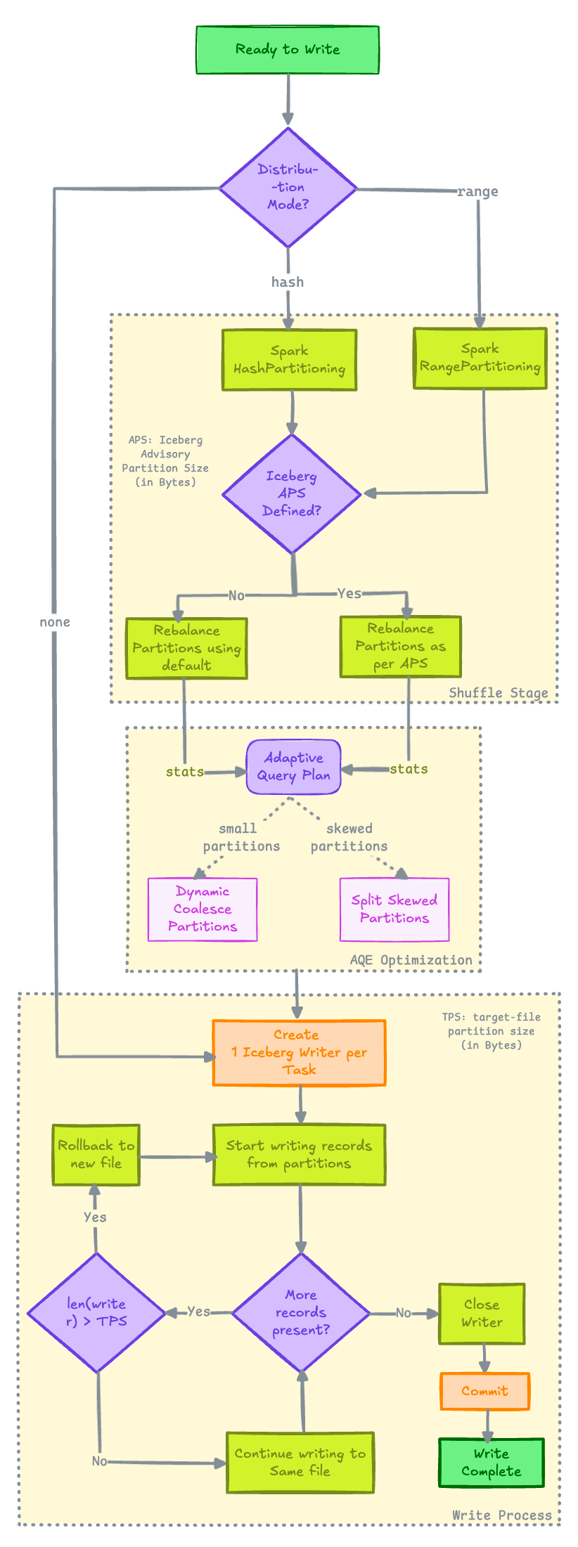
Here's a flow diagram that shows how everything explained so far works together
Final Thoughts
In my experience of migrating from Hive to Iceberg Table Format, if you are looking to get the best write performance out of your jobs with Iceberg, you need to find a balance between performance and the file size.
If you have followed until here, you have a solid foundation good to go run some tests for your use case and figure out the configurations that suits best for usecase.
Got more questions on this? Feel free to drop those in the comments section.
If you are interested in the code on how to run your tests, or need to see some proof of what we have discussed here, next section covers it all.
How can I run tests?
If this is something that you are wondering, this will give you a quick start, I will be using Spark 3.5.3 with Iceberg 1.5.0 (similar to AWS EMR 7.2). For this post, I am running these tests on a Spark Standalone Cluster running on my Mac M1 with MinIO as object storage.
You can pick your cloud vendor, change the configurations for Spark initialization and run these tests with APS and other configurations modified.
Initializing Spark Session
from pyspark.sql import SparkSession
import os

ICEBERG_CATALOG = "ic_minio"
DW_PATH = 's3a://warehouse/iceberg'

spark = SparkSession.builder \
    .master("spark://spark-master:7077") \
    .appName("spark-minio") \
    .config("spark.eventLog.enabled", "true")\
    .config("spark.eventLog.dir", "/opt/spark/spark-events")\
    .config("spark.history.fs.logDirectory", "/opt/spark/spark-events")\
    .config('spark.jars', '/opt/extra-jars/iceberg-spark-runtime-3.5_2.12-1.5.0.jar,/opt/extra-jars/hadoop-aws-3.3.4.jar,/opt/extra-jars/aws-java-sdk-bundle-1.12.262.jar')\
    .config("spark.hadoop.fs.s3a.endpoint", os.environ.get('MINIO_ENDPOINT')) \
    .config("spark.hadoop.fs.s3a.access.key", os.environ.get('MINIO_ACCESS_KEY')) \
    .config("spark.hadoop.fs.s3a.secret.key", os.environ.get('MINIO_SECRET_KEY')) \
    .config("spark.hadoop.fs.s3a.path.style.access", "true") \
    .config("spark.hadoop.fs.s3a.impl", "org.apache.hadoop.fs.s3a.S3AFileSystem") \
    .config("spark.hadoop.fs.s3a.aws.credentials.provider", "org.apache.hadoop.fs.s3a.SimpleAWSCredentialsProvider") \
    .config(f'spark.sql.catalog.{ICEBERG_CATALOG}','org.apache.iceberg.spark.SparkCatalog') \
    .config(f'spark.sql.catalog.{ICEBERG_CATALOG}.type','hadoop') \
    .config(f'spark.sql.catalog.{ICEBERG_CATALOG}.warehouse', DW_PATH) \
    .getOrCreate()
SparkSession initialization with MinIO as Object Storage
Creating Table using NYC dataset for running tests
from pyspark.sql.functions import lit, col

# Creating table
yellow_taxi_table = f"{ICEBERG_CATALOG}.db.yellow_taxi"

df = spark.read.parquet("s3a://warehouse/raw_data/nyc_taxi/yellow_taxi/2023/")
df = df.withColumn("year", lit(2023))

# Creating a table partitioned on `year` column
df.writeTo(yellow_taxi_table).partitionedBy("year").create()

# time taken: 22secs
Creating yellow_taxi table to run tests
Let's look into metadata tables, to set the baseline for our tests.
def show_num_files_added_deleted():
  spark.table(f"{yellow_taxi_table}.manifests")\
      .select("content",
        "path",
        "added_snapshot_id",
        "added_data_files_count",
        "deleted_data_files_count").show()

show_num_files_added_deleted()
Checking number of data_files added or deleted
+-------+--------------------+-------------------+----------------------+------------------------+
|content|                path|  added_snapshot_id|added_data_files_count|deleted_data_files_count|
+-------+--------------------+-------------------+----------------------+------------------------+
|      0|s3a://warehouse/i...|8588694681592483501|                     1|                       0|
+-------+--------------------+-------------------+----------------------+------------------------+
Output of manifests metadata table
# Checking the file sizes of the data files
from pyspark.sql.functions import round

def show_file_sizes():
  spark.table(f"{yellow_taxi_table}.files")\
      .select("content",
        "file_path",
        "partition",
        "file_size_in_bytes")\
      .withColumn("file_size_in_mb", lit(round(
          col("file_size_in_bytes")/(1024*1024), 2)))\
      .show()

show_file_sizes()
Querying files metadata table to check the file size
-------+--------------------+---------+------------------+---------------+
|content|           file_path|partition|file_size_in_bytes|file_size_in_mb|
+-------+--------------------+---------+------------------+---------------+
|      0|s3a://warehouse/i...|   {2023}|         101068454|          96.39|
+-------+--------------------+---------+------------------+---------------+
1 Data Files written of size 96.39MB
Alright now, we have a baseline set with default configurations. Time to run some tests.
Test #1: Distribution mode none
# Setting distribution mode as none

df.withColumn("year", lit(2023))\
    .writeTo(yellow_taxi_table)\
    .option("distribution-mode", "none")\
    .overwrite(col("year") == 2023)

# Time taken: 17secs
Re-writing same data with distribution mode as none
# Checking number of files written

show_num_files_added_deleted()
Querying manifest metadata table
+-------+--------------------+-------------------+----------------------+------------------------+
|content|                path|  added_snapshot_id|added_data_files_count|deleted_data_files_count|
+-------+--------------------+-------------------+----------------------+------------------------+
|      0|s3a://warehouse/i...|7240009054708452262|                     7|                       0|
|      0|s3a://warehouse/i...|7240009054708452262|                     0|                       1|
+-------+--------------------+-------------------+----------------------+------------------------+
7 Data Files written and 1 Data Files Deleted
# Checking file sizes

show_file_sizes()
Querying files metadata table to check the file sizes
+-------+--------------------+---------+------------------+---------------+
|content|           file_path|partition|file_size_in_bytes|file_size_in_mb|
+-------+--------------------+---------+------------------+---------------+
|      0|s3a://warehouse/i...|   {2023}|          16896993|          16.11|
|      0|s3a://warehouse/i...|   {2023}|          16718982|          15.94|
|      0|s3a://warehouse/i...|   {2023}|          12116148|          11.55|
|      0|s3a://warehouse/i...|   {2023}|          16710019|          15.94|
|      0|s3a://warehouse/i...|   {2023}|          16489463|          15.73|
|      0|s3a://warehouse/i...|   {2023}|          16604224|          15.84|
|      0|s3a://warehouse/i...|   {2023}|           6703050|           6.39|
+-------+--------------------+---------+------------------+---------------+
File sizes of 7 generated files
In case, you are wondering why there is 1 data file deleted, it's because the table we have created by default is a Copy-on-Write table.
If you are new to COW and MOR materialization in Apache Iceberg, you can read through this post:

Test #1.1 Distribution Mode none and APS = 64MB
Here we will test, if setting APS has any impact when distribution mode is none.
df.withColumn("year", lit(2023))\
    .writeTo(yellow_taxi_table)\
    .option("distribution-mode", "none")\
    .option("advisory-partition-size", "67108864")\
    .overwrite(col("year") == 2023)

# Time taken: 18secs
Re-writing same data with distribution mode as none and APS set as 64MB
show_num_files_added_deleted()Querying manifest metadata table
+-------+--------------------+-------------------+----------------------+------------------------+
|content|                path|  added_snapshot_id|added_data_files_count|deleted_data_files_count|
+-------+--------------------+-------------------+----------------------+------------------------+
|      0|s3a://warehouse/i...|4040802190445405605|                     7|                       0|
|      0|s3a://warehouse/i...|4040802190445405605|                     0|                       7|
+-------+--------------------+-------------------+----------------------+------------------------+
7 Data Files written and 7 Data Files Deleted
show_file_sizes()Querying files metadata table to check the file sizes
+-------+--------------------+---------+------------------+---------------+
|content|           file_path|partition|file_size_in_bytes|file_size_in_mb|
+-------+--------------------+---------+------------------+---------------+
|      0|s3a://warehouse/i...|   {2023}|          16896993|          16.11|
|      0|s3a://warehouse/i...|   {2023}|          16718982|          15.94|
|      0|s3a://warehouse/i...|   {2023}|          12116148|          11.55|
|      0|s3a://warehouse/i...|   {2023}|          16710019|          15.94|
|      0|s3a://warehouse/i...|   {2023}|          16489463|          15.73|
|      0|s3a://warehouse/i...|   {2023}|          16604224|          15.84|
|      0|s3a://warehouse/i...|   {2023}|           6703050|           6.39|
+-------+--------------------+---------+------------------+---------------+
File sizes of 7 generated files
No change in file sizes as expected – remember none mode has no shuffling involved, hence no impact of setting APS value. 7 files written are completely dependent on the number of tasks present in the stage before writing.
Test #2 Distribution Mode hash and Target File Size = 32MB
Here we will test how write times are impacted when TFS is set to 32MB.
# Writing files with 32MB

df.withColumn("year", lit(2023))\
    .writeTo(yellow_taxi_table)\
    .option("distribution-mode", "hash")\
    .option("target-file-size-bytes", "33554432")\
    .overwrite(col("year") == 2023)

# Time taken: 13secs
Re-writing same data with distribution mode as hash and TFS set as 32MB
show_num_files_added_deleted()Querying manifest metadata table
+-------+--------------------+-------------------+----------------------+------------------------+
|content|                path|  added_snapshot_id|added_data_files_count|deleted_data_files_count|
+-------+--------------------+-------------------+----------------------+------------------------+
|      0|s3a://warehouse/i...|8473979551813488551|                     3|                       0|
|      0|s3a://warehouse/i...|8473979551813488551|                     0|                       7|
+-------+--------------------+-------------------+----------------------+------------------------+
3 Data Files written and 7 Data Files Deleted
show_file_sizes()Querying files metadata table to check the file sizes
+-------+--------------------+---------+------------------+---------------+
|content|           file_path|partition|file_size_in_bytes|file_size_in_mb|
+-------+--------------------+---------+------------------+---------------+
|      0|s3a://warehouse/i...|   {2023}|          33651531|          32.09|
|      0|s3a://warehouse/i...|   {2023}|          33590979|          32.03|
|      0|s3a://warehouse/i...|   {2023}|          32854639|          31.33|
+-------+--------------------+---------+------------------+---------------+
File Sizes of 3 generated files
Test #3 Distribution Mode hash and APS = 128MB
Here we will test how write times are impacted when APS is set to 128MB, i.e., Default value mentioned in codebase.
df.withColumn("year", lit(2023))\
    .writeTo(yellow_taxi_table)\
    .option("distribution-mode", "hash")\
    .option("advisory-partition-size", "134217728")\
    .overwrite(col("year") == 2023)

  # Time taken: 9secs
Re-writing same data with distribution mode as hash and APS set as 128MB
show_num_files_added_deleted()Querying manifest metadata table
+-------+--------------------+-------------------+----------------------+------------------------+
|content|                path|  added_snapshot_id|added_data_files_count|deleted_data_files_count|
+-------+--------------------+-------------------+----------------------+------------------------+
|      0|s3a://warehouse/i...|7566709592861267832|                     3|                       0|
|      0|s3a://warehouse/i...|7566709592861267832|                     0|                       3|
+-------+--------------------+-------------------+----------------------+------------------------+
show_file_sizes()Querying files metadata table to check the file sizes
+-------+--------------------+---------+------------------+---------------+
|content|           file_path|partition|file_size_in_bytes|file_size_in_mb|
+-------+--------------------+---------+------------------+---------------+
|      0|s3a://warehouse/i...|   {2023}|          33059607|          31.53|
|      0|s3a://warehouse/i...|   {2023}|          28265100|          26.96|
|      0|s3a://warehouse/i...|   {2023}|          38595219|          36.81|
+-------+--------------------+---------+------------------+---------------+
Files Sizes when APS was set to 128MB
In Test#3, time taken is the least during writes, i.e., 9secs. That included shuffling because of Distribution Mode = hash. Interesting. right?
References
[1] waitingforcode.com AQE
[2] AdaptiveSparkPlanExec.scala
[3] Iceberg Write Properties Documentation
That's it for this one! 🚀 See you in the next one.
What issues did you run into after migration to Iceberg?
Got any more questions? Put it in the comments.


Member discussion